Context
In a particle physics experiment, a lot of data is produced and must be analyzed to extract useful information. This data typically consists of many independent observations of a “physics event” inside of some detector, which records information about the event. Often the analysis boils down to classifying a large dataset of events into a few categories, with the most simple example having only ‘signal’ and ‘background’ types of events. For instance, in a neutrinoless double beta decay ($0\nu\beta\beta$) experiment, the ‘signal’ would be the $0\nu\beta\beta$ events, while everything else (radioactive decay, solar neutrinos, $2\nu\beta\beta$, self destructing dark matter, etc.) would be backgrounds. Once the events have been classified, it is straightforward to turn numbers of events into (relative) rates or probabilities of each event class by taking ratios of the different classes. This higher level information can be be used to constrain (or disprove) theoretical models for how particles interact.
There are several methods for performing such a classification. Particle accelerator experiments like the LHC provide a lot of information about each event, and these experiments often write complicated algorithms to directly label each type of event as belonging to a certain class. Bolometer experiments like Cuore, which provide only information about the total energy of an event, and optical neutrino detectors like SNO+, which provide information about the position, energy, and perhaps direction of an event, often have to rely on statistical methods. This is largely due to the fact that the data collected is not sufficient to uniquely classify every even. For example, even if a signal occurs in a specific energy range, like $0\nu\beta\beta$, backgrounds, such as radioactive decay, can have very similar energies and be much more common. Detector energy resolutions complicate matters further by smearing out the measured energies relative to the true energies.
These statistical methods don’t directly classify any particular event, but can still give a high precision answer to the overall content of a large dataset. This is possible because events of different types tend to have different distributions. For instance, radioactive backgrounds will occur more frequently near areas higher in radioactivity, while solar neutrino interactions would tend to be uniformly distributed in a detector. Similarly signals like $0\nu\beta\beta$ will occur at discrete energies, while a background like $2\nu\beta\beta$ will have a wide distribution of energies with a known shape. As long as one accounts for all possible types of events present in a dataset and can reliably know how these events should be distributed as a function of some parameters, one can statistically extract the makeup of a dataset. The one caveat is that event classes have to look sufficiently different as a function of the parameters chosen.
Fully accounting for all possible event classes present in a dataset is no small task, and indeed this is one of the largest difficulties of any statistical analysis of this style. Choosing parameters is another difficulty. Energy is an obvious choice, since physical interactions typically have characteristic energy distributions, but this may not be sufficient to well-separate all event classes. The final big hurdle is knowing how the different event classes are distributed as a function of your chosen parameters. To do this, one must typically generate a fully calibrated simulation model where physical interactions can be simulated independently to generate a probability distribution function as a function of the chosen parameters for each class of events.
In the rest of this post, I will sketch out such an analysis using a maximum likelihood method with two classes of events and one parameter that can be compared to energy.
Maximum Likelihood Analysis
Start out with some basic imports to perform fast mathematical operations and generate plots in Python.
import numpy as np # Perform mathematical operations on arrays
from scipy.stats import poisson # To calculate poisson probabilities
import scipy.optimize as opt # Function optimizers and root finders
import matplotlib.pyplot as plt # Creating plots

#Force matplotlib to make Pretty Plots™
import matplotlib
matplotlib.rcParams['figure.figsize'] = [10,7]
matplotlib.rcParams['xtick.top'] = True
matplotlib.rcParams ['xtick.direction'] = 'in'
matplotlib.rcParams['xtick.minor.visible'] = True
matplotlib.rcParams['ytick.right'] = True
matplotlib.rcParams['ytick.direction'] = 'in'
matplotlib.rcParams['ytick.minor.visible'] = True
matplotlib.rcParams['font.size'] = 19
matplotlib.rcParams['font.family']= 'DejaVu Serif'
matplotlib.rcParams['mathtext.default'] = 'regular'
matplotlib.rcParams['errorbar.capsize'] = 3
matplotlib.rcParams['figure.facecolor'] = (1,1,1)
This will be a one dimensional analysis, i.e. one parameter will be used to distinguish event classes. More dimensions will likely enhance the ability to distinguish events, but higher dimensions require more simulated data, more processing time, and more complicated code. Higher dimensions use the same basic framework though, hence a one dimensional example is a good starting point. Now choose and region of interest (ROI) for this analysis on the chosen dimension. We’ll be working with totally made-up events as you see, but let’s assume they’re distributed in the low tens of mega electronvolts.
binning = np.linspace(0,25,40) # 40 bins from 0 to 25 MeV
Now create a Monte-Carlo (MC) simulation model for two classes of events. Reality here is much more complicated, but for the purposes of this demonstration, assume:
- Class A has a mean energy of 10 MeV and is described by a Gaussian distribution with width 2 MeV
- Class A has a mean energy of 15 MeV and is described by a Gaussian distribution with width 3 MeV Generate 10000 of these events for building PDFs for these classes later.
# precision monte carlo simulation :)
def class_a(nev):
    return np.random.normal(10,2,size=nev)
def class_b(nev):
    return np.random.normal(15,3,size=nev)

# generate and save 10000 MC events for each class
mc_class_a = class_a(10000)
mc_class_b = class_b(10000)

plt.hist(mc_class_a,bins=binning,histtype='step',label='Class A')
plt.hist(mc_class_b,bins=binning,histtype='step',label='Class B')
plt.xlabel('Energy (MeV)')
plt.legend()
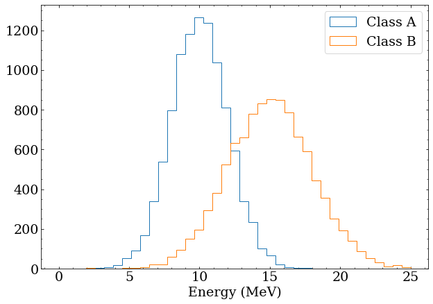
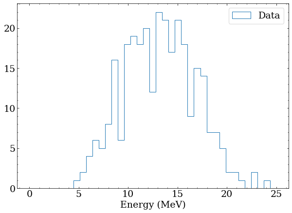
Note that these distributions overlap significantly, and particularly for events in the 10-15 MeV range, it would be impossible on an event-by-event basis to distinguish the two classes. To make this more obvious, generate a fake sample of data with 100 class A and 200 class B events. This is a stand in for real data, and testing an analysis with artificially constructed datasets is an important step in any real analysis.
# a fake dataset containing 100 class A and 200 class B
data = np.concatenate([class_a(100),class_b(200)])

plt.hist(data,bins=binning,histtype='step',label='Data')
plt.xlabel('Energy (MeV)')
plt.legend()
Binned likelihood function
To determine the number of each class of event in the data, a likelihood function needs to be constructed and optimized. This function will be parameterized by a hypothesized number of events for each event class $\mu_j$ for class $j$. A binned fit will be performed, so this function will need to construct an expected number of events for each bin according to the expected distributions for each class. This is particularly useful when you have a large amount of data, since it is less computationally intense than an unbinned fit. An unbinned fit is certainly possible, and can be thought of as letting the bin width go to zero. This may be necessary if your PDFs are not smooth compared to the size of your bins.
To do a binned fit, the simulated datasets for class A and B will be binned and normalized, then the bins will be scaled by the hypothesized number of events for each class. Mathematically, bin $i$ of the normalized PDFs for each event class $j$ can be written as $H_{ji}$. So the expected number of events in each bin, $\lambda_i$, can be written as:
$$ \lambda_i = \sum_j \mu_j H_{ij} $$
Finally, the Poisson likelihood ${\scr L}_i$ of observing the number of data events in each bin $k_i$ will be calculated according to the calculated expected events $\lambda_i$
$$ {\scr L}_i = \frac{{\lambda_i}^{k_i}e^{-\lambda_i}}{k_i!} $$
You may be tempted to directly calculate this using power, exp, and factorial functions - don’t!
Both the power and the factorial will overflow easily for even moderately sized datasets.
Fortunately in python, the scipy.stats.poisson module provides a pmf (PDF) function that calculates this without having to worry about intermediate large numbers.
Finally, to arrive at the total likelihood $\scr L$, the product of the likelihood of each bin is multiplied together
$$ {\scr L} = \prod_i {\scr L}_i $$
All of this is encapsulated in a Python class where the __init__ method performs the initial setup and a __call__ method evaluates the likelihood function.
class LikelihoodFunction:

    def __init__(self,data,event_classes,binning):
        '''Sets up a likelihood function for some data and event classes

           data is a 1D array of quantities describing each data event
           event_classes is a list of 1D arrays with quantites for each event
               class. These should be derived from simulation, and will be
               used to generate PDFs for each event class.
           binning is a 1D array of bin edges describing how the data and PDFs
               should be binned for this analysis.
        '''
        # First step is to bin the data into a histogram (k_i)
        self.data_counts = np.histogram(data,bins=binning)[0]
        # Create a list to store PDFs for each event class
        self.class_pdfs = []
        for event_class in event_classes:
            # Bin the MC data from each event class the same way as data
            pdf_counts = np.histogram(event_class,bins=binning)[0]
            # Normalized PDF (H_ij) such that sum of all bins is 1
            pdf_norm = pdf_counts/np.sum(pdf_counts)
            # Save for later
            self.class_pdfs.append(pdf_norm)

    def __call__(self,*params):
        '''Evaluates the likelihood function and returns likelihood

           params is a list of scale factors for each PDF (event_class) passed
               to the __init__ method.
        '''
        # Observed event histogram is always the binned data
        observed = self.data_counts
        # Expected events are normalized PDFs times scale factors (\mu_j) for each PDF
        expecteds = [scale*pdf for scale,pdf in zip(params,self.class_pdfs)]
        # Sum up all the expected event historgrams bin-by-bin (sum over j is axis 0)
        expected = np.sum(expecteds,axis=0)
        # Calculate the bin-by-bin poisson probabilities to observe `observed` events
        # with an average `expected` events in each bin (these poisson functions operate bin-by-bin)
        bin_probabilities = poisson.pmf(observed,expected)
        # multiply all the probabilities together
        return np.prod(bin_probabilities)
Using the fake data and MC generated above, this class can be used to create a likelihood function:
# Build the likelihood function for the data and with our two event classes and binning
lfn = LikelihoodFunction(data,[mc_class_a,mc_class_b],binning)
This likelihood function can be __call__ed to calculate the likelihood for some scale factors.
Here the ’true’ scale factors are passed to see their likelihood.
print(lfn(100,200))
Results:
2.517486079648127e-31
Note that these likelihoods are typically tiny. With many bins, you can easily run out of precision even with 64bit float values, which is one reason people tend to work with the logarithm of the likelihood (next section) instead.
Likelihood space
The likelihood function here is a two parameter function because two event classes were used.
It calculates the likelihood (probability) of observing the data given the expected (MC simulated) event classes scaled by factors that represent the number of events of each class in the dataset.
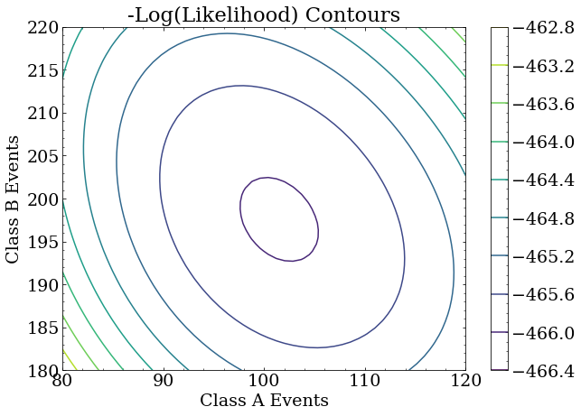
Because this is a 2D likelihood space, we can make a nice contour plot of the likelihood as a function of the two scale factors around where we constructed the true answer to be: (100,200).
#A numpy recipe for creating a 2D grid
X,Y = np.meshgrid(np.linspace(80,120),np.linspace(180,220))
#Evaluate the likelihood at each point on the grid
Z = [lfn(x,y) for x,y in zip(X.flatten(),Y.flatten())]
#Reshape the Z result to match the recipe shapes so plotting functions can use it
Z = np.asarray(Z).reshape(X.shape)

plt.contour(X,Y,Z)
plt.colorbar()
plt.title('Likelihood Contours')
plt.xlabel('Class A Events')
plt.ylabel('Class B Events')
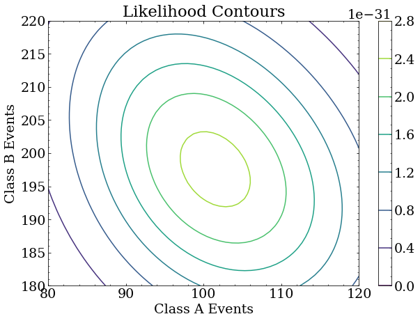
Note that the largest likelihood is, in fact, near the true answer. It is not exactly at the true answer because this is a small data set used for this exercise, and the statistical uncertainty of the analysis is correspondingly large. With more data, the maximum likelihood will be arbitrarily close to the true answer. With different data of the same size as this exercise, the maximum likelihood point will fluctuate around the true answer.
Maximum likelihood
It is now a computational exercise to find the point of maximum likelihood.
Typically, function optimizers are designed to find minimum values, and it is trivial to adapt our likelihood to this domain: simply minimize the negative likelihood to find the maximum likelihood.
The scipy.optimize.minimize routine encapsulates several robust optimizers.
Here, I have opted to use the Nelder-Mead simplex method which is a good general purpose algorithm that makes very few assumptions about the function it is minimizing, and works well even with higher dimensional and rough functions.
# Many minimizers require an initial guess (50,50)
# for smooth functions with one global minimum, this need not be a good guess
result = opt.minimize(lambda x: -lfn(*x),x0=(50,50),method='Nelder-Mead')

# Note fun (minimum value), nfev (number of times lfn function called), and x (the minimum location)
print(result)
Results:
 final_simplex: (array([[101.45923284, 197.54074435],
       [101.45923555, 197.54080241],
       [101.45933045, 197.5406877 ]]), array([-2.55289889e-31, -2.55289889e-31, -2.55289889e-31]))
           fun: -2.5528988901237637e-31
       message: 'Optimization terminated successfully.'
          nfev: 110
           nit: 56
        status: 0
       success: True
             x: array([101.45923284, 197.54074435])
This indicates the point of maximum likelihood is (101,197) which is quite close to the true value for this data set.
You could go on from here to integrate the likelihood around this point to find a region containing e.g. $0.95$ total probability, which would give a 95% confidence limit interval.
For problems that are sufficiently close to having Gaussian errors (likelihood described well by a Gaussian distribution), there are easier methods using the negative logarithm of the likelihood.
Binned negative log likelihood function
To avoid very small numbers in likelihoods, one can opt to minimize the negative logarithm of the likelihood instead. This can also simplify the procedure of finding confidence intervals significantly. To start, first examine the Poisson likelihood ${\scr L}_i$ for one bin in the histogram, with $k_i$ observed events and an expected number of events $\lambda_i$
$$ {\scr L}_i = \frac{{\lambda_i}^{k_i}e^{-\lambda_i}}{k_i!} $$
The negative logarithm of this, expanded out is
$$ -\log{{\scr L}_i} = \lambda_i - k_i \log{(\lambda_i}) + \log{(k_i !)} $$
The observed events $k_i$ is a constant in the likelihood function, while the $\lambda_i$ is constructed from the PDFs and changes with the scale factors, which are the parameters of the likelihood function and change. This means the final term $\log{(k_i !)}$ is a constant term and only shifts the likelihood function, so these terms can be omitted during the optimization process without affecting the minimum found. I’ll use ${\cal L}_i$ to refer to this modified negative log likelihood.
$$ {\cal L}_i = \lambda_i - k_i \log{(\lambda_i}) $$
The total negative log likelihood $\cal L$ is now given by the sum of ${\cal L}_i$ for all bins
$$ {\cal L} = \sum_i {\cal L}_i $$
This can be implemented in a very similar Python class:
class NegativeLogLikelihoodFunction:

    # This is the same as before
    def __init__(self,data,event_classes,binning):
        self.data_counts = np.histogram(data,bins=binning)[0]
        self.class_pdfs = []
        for event_class in event_classes:
            pdf_counts = np.histogram(event_class,bins=binning)[0]
            pdf_norm = pdf_counts/np.sum(pdf_counts)
            self.class_pdfs.append(pdf_norm)

    def __call__(self,*params):
        observed = self.data_counts
        expecteds = [scale*pdf for scale,pdf in zip(params,self.class_pdfs)]
        expected = np.sum(expecteds,axis=0)
        # Calculate the bin-by-bin -log(poisson probabilities) sans constant terms
        # Note, regions in your ROI with no expected counts (0 bins in PDF) must be excluded
        mask = expected > 0
        bin_nlls = expected[mask]-observed[mask]*np.log(expected[mask])
        # multiply all the probabilities -> add all negative log likelihoods
        return np.sum(bin_nlls)
And a negative log likelihood function can be constructed in the same way as the likelihood function:
nllfn = NegativeLogLikelihoodFunction(data,[mc_class_a,mc_class_b],binning)
Negative log likelihood space
A contour plot again shows that the largest likelihood is in the same place as before.
Minimum negative log likelihood
Further, minimizing this function gives the same result as before:
# Minimize like before
nll_result = opt.minimize(lambda x: nllfn(*x),x0=(50,50),method='Nelder-Mead')

# Note fun (minimum value), nfev (number of times lfn function called), and x (the minimum location)
print(nll_result)
Results:
 final_simplex: (array([[101.45923284, 197.54074435],
       [101.45923555, 197.54080241],
       [101.45933045, 197.5406877 ]]), array([-466.04590926, -466.04590926, -466.04590926]))
           fun: -466.0459092567508
       message: 'Optimization terminated successfully.'
          nfev: 110
           nit: 56
        status: 0
       success: True
             x: array([101.45923284, 197.54074435])
Confidence intervals
Finding a maximum likelihood is not the end of an analysis. One also needs to understand the statistical uncertainty in the optimal parameters. As mentioned earlier, the likelihood function represents probabilities for a particular set of parameters, so integrating the likelihood function in a region directly gives the probability that the answer lies in that region. Poisson likelihoods, as we are dealing with here, are incidentally closely related to the $\chi^2$ statistic. As is shown by Wilks’ theorem, $-2$ times the logarithm of a likelihood ratio (where one likelihood represents a null hypothesis (the best-fit) and another likelihood is for an alternative set of parameters) is approximately Chi-squared distributed for sufficiently large datasets (where statistical error is small and the likelihood is well described by a Gaussian distribution).
$$ \chi^2 = -2 \log \frac{ {\scr L}_{alt} }{ {\scr L} } $$
Or, for the notation used for negative log likelihood:
$$ \chi^2 = 2 ({\cal L}_{alt} - {\cal L}) = 2 \Delta {\cal L} $$
So, a difference in log likelihood can use to get a $\chi^2$ p-value, which can be used to set a confidence limit. This means a one-sigma confidence for one parameter ($\chi^2$ of $1$) corresponds to $\Delta {\cal L} = \frac{1}{2}$.
To arrive at this $\Delta {\cal L}$ value, it is easiest to “profile” the likelihood, which means scanning one parameter while maximizing the likelihood (floating) the other parameters. A more mathematically rigorous approach again involves integrating the likelihood directly to “marginalize” away other variables. Python code for functions that returned the profiled negative log likelihood for the class A and B scale factors is as follows:
def profile_class_a(nev):
    '''Profile away class_b scale factor to get 1D delta NLL for class_a'''
    return opt.minimize(lambda x: nllfn(nev,x[0]),x0=(50,),method='Nelder-Mead').fun - nll_result.fun
def profile_class_b(nev):
    '''Profile away class_a scale factor to get 1D delta NLL for class_b'''
    return opt.minimize(lambda x: nllfn(x[0],nev),x0=(50,),method='Nelder-Mead').fun - nll_result.fun
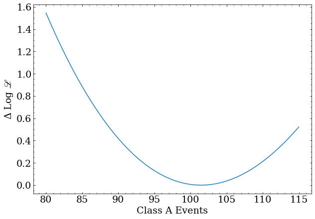
The profile for the class A scale factor:
x = np.linspace(80,115,50)
y = [profile_class_a(nev) for nev in x]
plt.plot(x,y)
plt.xlabel('Class A Events')
plt.ylabel('-$\Delta$ Log ${\scr L}$')
The profile for the class B scale factor:
x = np.linspace(180,215,50)
y = [profile_class_b(nev) for nev in x]
plt.plot(x,y)
plt.xlabel('Class B Events')
plt.ylabel('$\Delta$ Log ${\scr L}$')

It is then easy to use a root finding algorithm to look for the where these functions cross $\frac{1}{2}$
def confidence_interval(delta_nll_fn,central,step):
    ''' Finds 1sigma confidence interval for a delta_nll_fn of one parameter
        around a central value with a max distance of step.'''
    lo = opt.brentq(lambda x: delta_nll_fn(x)-0.5,central-step,central)
    hi = opt.brentq(lambda x: delta_nll_fn(x)-0.5,central,central+step)
    return lo,hi

central = nll_result.x[0]
lo,hi = confidence_interval(profile_class_a,central,50)
print('Number of A events = $%0.2f^{+%0.2f}_{-%0.2f}$'%(central,hi-central,central-lo))

central = nll_result.x[1]
lo,hi = confidence_interval(profile_class_b,central,50)
print('Number of B events = $%0.2f^{+%0.2f}_{-%0.2f}$'%(central,hi-central,central-lo))
Number of A events = $ 101.46^{+13.24}_{-12.49} $
Number of B events = $ 197.54^{+16.56}_{-15.78} $
These results are nicely consistent with the initial conditions, as the estimated parameter error covers the true value. To demonstrate a rigorous fit, one would repeat this procedure for many different fake datasets and record the results. The results of this meta-analysis can be used to demonstrate both that the one-sigma confidence intervals actually contain the true values the correct fraction of the time and that there is no bias between the true and estimated number of events on average.
Final Results
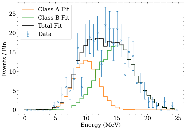
The fitted number of events can be used to generate the $\lambda_i$ expected events for each bin, as well as the breakdown by event class. It is straightforward to plot this, both to demonstrate that the best fit agrees well with the data, and show how the total fit is built from the PDFs of the event classes. This is done with the following Python code, which also shows the data with Poisson error bars.
#Plot binned data with errorbars
bin_centers = (binning[:-1] + binning[1:])/2
plt.errorbar(bin_centers,nllfn.data_counts,yerr=np.sqrt(nllfn.data_counts),marker='x',linestyle='none',label='Data')
#Borrowed from the NegativeLogLikelihoodFunction class
expecteds = [scale*pdf for scale,pdf in zip(nll_result.x,nllfn.class_pdfs)]
#Plot each event class as a separate hisotgram
for class_name,expected_class in zip(['A','B'],expecteds):
    plt.plot(binning[:-1],expected_class,drawstyle='steps-post',label='Class %s Fit'%class_name)
#Sum the histograms to plot the total fit
expected = np.sum(expecteds,axis=0)
plt.plot(binning[:-1],expected,drawstyle='steps-post',color='k',label='Total Fit')
plt.legend()