Neutrino detector often detect neutrino indirectly by recording information about photons produced in the neutrino interaction. Simulations are used to understand how light propagates through the detector, and this allows one to understand the kinds of optical signals produced by different types of interactions. Many techniques can be exploited to maximize the amount of information detected, but ultimately the data boils down to the time at which photons are detected on light-sensitive elements in the detector. These light sensitive elements could be photomultiplier tubes (PMTs), large area picosecond photodetectors (LAPPDs), silicon photomultipliers (SiPMs), or something more exotic. All ultimately produce some electrical pulse, which is measured as a time-varying voltage.
Single photons
Particular photon detectors will have different pulse shapes, but all are well approximated by Log-normal distributions of the form $$ V(t|t_0,\mu,\sigma) = \frac{A}{t-t_0} \exp \left(-\frac{\ln (t-t_0) - \mu}{2\sigma^2} \right) $$ where $t_0$ is the arrival time of the photon, $A$ is a scale factor, $\mu$ and $\sigma$ are parameters that control the shape of the pulse.
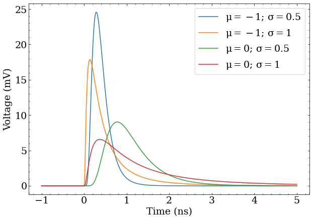
Several Log-normal pulse shapes, representative of the voltage signals produced by fast photon detectors. Absolute scale is approximately correct for the response to single photons.
The total integral, or charge, of a pulse produced by a single photon on a detector will follow some distribution, however the normalized pulse shape is typically very consistent between different pulses. This means by examining the pulse shape, one can very accurately determine the time at which a photon was detected. Even a simple method of calculating the time at which the pulse crosses some voltage threshold can achieve time resolutions of better than 1 ns for PMTs or 50 ps for LAPPDs.
Multiple photons
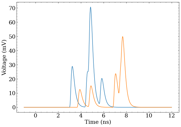
Two different traces with 5 pulses spread out in time. When they happen to be close together, they can be indistinguishable from a single pulse. Another set of traces with 5 pulses spread out in time. As the density increases, it’s even harder to distinguish individual pulses.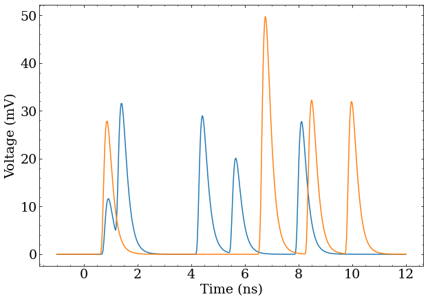
When there is the possibility of detecting multiple photons close together in time, a simple voltage threshold does not capture much of the available information. A minimal extension would be to integrate the region of many pulses. The integrated charge would be proportional to the detected number of photons, since the area of each pulse follows a distribution with some mean value. However, this approach provides no information about the arrival time of the remaining photons.
Often for neutrino detectors, the most critical information to obtain is the arrival time of the first photon, and the total number of detected photons. The former can be used for time of flight position reconstruction algorithms while the latter is proportional to the energy of the interaction. All the same, reconstruction would be significantly improved by obtaining the arrival times of all detected photons. Further, the charge distribution response to single photons can be broad (especially for PMTs), which means the total charge does not exactly determine the number of detected photons. Being able to count photons directly would provide better information than dividing the total charge by the mean charge.
The example figures show some cases where multiple photons are detected close together in time. One might be tempted to count peaks, but this does not work well when photons arrive close together in time. More complicated schemes of computing multiple thresholds, measuring pulse properties, or otherwise massaging these voltage traces, could be considered, but when the pulse shape is the same up to some scale factor, and one wants to know where (when), and how many, pulses are present in a signal, deconvolution is the only game in town.
(De)convolution
To understand deconvolution, one must first understand its inverse convolution. Conceptually, convolution smears out one function $f(t)$ by another function $g(t)$. Mathematically this is achieved by defining the value of the convolved function at a point $t$, written as $(f \ast g)(t)$ as the integral of the product of the function $f$ in the neighborhood of $t$ with a (reversed) copy of $g$ centered at that point $t$. $$ (f \ast g)(t) = \int f(t-u)g(u) \, du $$ To illustrate this, consider a delta function $\delta(x)$ defined as being only nonzero at zero and having an integral of 1. $$ \int \delta(x) dx = 1 $$ Such a function can be imagined as starting with a normalized Gaussian distribution, and letting its width go to zero. $$ \delta(x) \approx \lim_{\sigma \rightarrow 0} \frac{1}{\sigma\sqrt{2\pi}} e^{-\frac{x^2}{2\sigma^2}} $$ Then define a function $p(t) = \delta(t-a)$. Convolving some function $f(t)$ with $p(t)$ results in a copy of $f(t)$ displaced by $a$. $$ (f \ast p)(t) = \int f(t-u)\delta(u-a) \, du = f(t-a) $$ This is because $\delta(u-a)$ is only nonzero, and has an integral of 1, when $u = a$.
Building a series of pulses
One can then imagine a more complicated function with several delta functions, $q(t) = \sum_i \delta(t-a_i)$. Convolving some function $f(t)$ with $q(t)$ results in a a sum of $f(t)$ displaced by all the $a_i$. $$ (f \ast q)(t) = \int f(t-u)\sum_i\delta(u-a_i) \, du = \sum_i f(t-a_i) $$
In the last example, $q(t)$ can be thought of as an expression representing the arrival times of several photons $a_i$. If $f(t)$ is equated with the pulse shape of a single detected photon, then $(f \ast q)(t)$ is the total voltage response of the photodetector. With this intuition, photon detectors can be thought of as devices that perform a convolution. To then extract the arrival times of the photons, no matter how many there are or how much they overlap, one simply needs to undo the convolution.
Fourier transformations
To undo the convolution, one has to think of things a bit differently, and dive into Fourier transformations. Consider the Fourier transformation of $f(t)$: $$ \mathcal{F}\{f(t)\} = F(f) = \int f(t) e^{-2\pi i f t} \, dt = \int f(t) (\cos(2\pi f t) - i \sin(2\pi f t)) \, dt $$ which represents the phase and amplitude (as a complex number) of each sinusoidal frequency $f$ making up the function $f(t)$. Notably, a Fourier transformation can be undone by a very similar operation on $F(f)$: $$ \mathcal{F}^{-1}\{F(f)\} = f(t) = \int F(f) e^{2\pi i f t} \, df = \int F(f) (\cos(2\pi f t) + i \sin(2\pi f t)) \, df $$ That this is the inverse operation isn’t too hard to demonstrate: $$ \begin{aligned} f(t) &= \int F(f) e^{2\pi i f t} \, df \\ &= \int \left( \int f(\tau) e^{-2\pi i f \tau} \, d\tau \right) e^{2\pi i f t} \, df \end{aligned} $$ Note that $\tau$ is used instead of $t$ when the expression for $F(f)$ is substituted, because $t$ already appears in the expression. Rearranging this, one arrives at the following, which appears daunting at first glance. $$ \begin{aligned} f(t) &= \int \int f(\tau) e^{2\pi i f t} e^{-2\pi i f \tau} \, df d\tau \\ &= \int \int f(\tau) e^{2\pi i f (t-\tau)} \, df d\tau \end{aligned} $$ However, note that the exponential parts are oscillatory $\sin$ and $\cos$ functions, which integrate to zero on their own. If you’re not familiar with imaginary exponential, this is perhaps a bit easier to see if it’s expanded out as was done in the definitions of Fourier transformations above. $$ \begin{aligned} f(t) &= \int \int f(\tau) (\cos(2\pi f (t-\tau)) + i\sin(2\pi f (t-\tau)) \, df d\tau \\ f(t) &= \int f(\tau) \left( \int (\cos(2\pi f (t-\tau)) + i\sin(2\pi f (t-\tau)) \, df \right) d\tau \\ \end{aligned} $$ Note that each term is the $\sin$ or $\cos$ of a difference of two angles. If the arguments to the functions are different ($t$ vs $\tau$) each term is an oscillatory function about zero, so its total integral over $f$ is zero. With $t = \tau$, the part in the innermost integral simplifies to $1$, since $t-\tau = 0$, meaning that innermost integral is (technically) infinite when $t = \tau$. This ultimately means the $\int e^{2\pi i f (t -\tau)} \, df$ part of the expression above acts like a delta function $\delta(t-\tau)$. (As a physicist, I would handwave that an infinite integral times an infinitesimal $d\tau \approx \frac{1}{\infty}$ is approximately 1 — mathematicians undoubtedly have a more rigorous definition.) We are left with the following, which has already been solved by considering delta functions, above. $$ f(t) = \int f(\tau) \delta(t-\tau) \, d\tau = f(t) $$
Fourier transformations are useful in many areas of mathematical analysis, as operations that are complicated in the time-domain $f(t)$ can be much simpler in the frequency domain $F(f)$. That’s certainly the case for convolutions.
Convolutions in the frequency domain
Consider the definition of a convolution, copied from above. $$ (f \ast g)(t) \int f(t-u)g(u) \, du $$ If $f(t)$ is defined in terms of its Fourier transform $\mathcal{F}\{f(t)\} = F(f)$, then $$ f(t) = \mathcal{F}^{-1}\{F(f)\} = \int F(f) e^{2\pi i f t} \, df $$ and this can be substituted into the definition of the convolution, and massaged a bit. $$ \begin{aligned} (f \ast g)(t) &= \int \left( \int F(f) e^{2\pi i f (t-u)} \, df \right) g(u) \, du \\ &= \int \int F(f) e^{2\pi i f (t-u)} g(u) \, df du\\ &= \int \int F(f) e^{2\pi i f t} e^{-2\pi i f u} g(u) \, df du \\ &= \int F(f) \left(\int g(u) e^{-2\pi i f u} \, du \right) e^{2\pi i f t} \, df \end{aligned} $$ Now recognize that the part in parentheses is the Fourier transform of $g(t)$. $$ G(f) = \mathcal{F}\{g(t)\} = \int g(t) e^{-2\pi i f t} \, dt $$ After that substitution, one has $$ (f \ast g)(t) = \int F(f) G(f) e^{2\pi i f t} \, df $$ which is the inverse Fourier transform of the product of $F(f)G(f)$! $$ \begin{align} (f \ast g)(t) &= \mathcal{F}^{-1}\{ F(f)G(f) \} \\ \mathcal{F} \{ (f \ast g)(t) \} &= F(f)G(f) \end{align} $$ So, the relatively complicated convolution operation on two functions is simply a multiplication of their Fourier transformations, followed by an inverse Fourier transformation.
Deconvolution in the frequency domain
If a convolution is a multiplication, then its inverse is necessarily a division, just in the frequency domain instead of the time domain. If $h(t)$ is defined as the convolution of signal $f(t)$ and some response function $g(t)$, with Fourier transforms $H(f)$, $F(f)$, and $G(f)$, respectively $$ \begin{aligned} h(t) &= (f \ast g)(t) = \mathcal{F}^{-1}\{ F(f)G(f) \} \\ \implies H(f) &= F(f)G(f) \end{aligned} $$ Then the following is true $$ F(f) = H(f) / G(f) $$ and one can recover $f(t)$ from $h(t)$ and $g(t)$. $$ f(t) = \mathcal{F}^{-1}\{ \mathcal{F}\{h(t)\} / \mathcal{F}\{g(t)\} \} $$ This, finally, presents a method for deconvolving a signal, provided that Fourier transformations of a measured signal are possible.
One may not want to Fourier transform all data in order to deconvolve it, as this can be an expensive, or hard to implement. Fortunately, the duality between convolution in the time domain and multiplication in the frequency domain can again be exploited. $$ \begin{aligned} f(t) &= \mathcal{F}^{-1}\{ \mathcal{F}\{h(t)\} \times \frac{1}{\mathcal{F}\{g(t)\}} \} \\ &= ( h \ast \mathcal{F}^{-1}\{ \frac{1}{G(f)}\})(t) \end{aligned} $$ If the function $k(t)$ is defined as the inverse Fourier transform of the inverse of the Fourier transform of $g(t)$ (call this last inverse $K(f)$, following the notation in this section), then this simplifies to a single convolution. $$ f(t) = (h \ast k)(t) $$
Not-so-ideal delta functions
What might not be obvious here is that the definition of $K(f)$ $$ K(f) = \frac{1}{G(f)} $$ is really the ratio of the Fourier transform of the delta function ($\mathcal{F}\{\delta(t)\} = 1$) to the Fourier transform of the convolution function $g(t)$. This has the effect of transforming structures like $g(t)$ into delta functions, which is mathematically ideal, but has the undesirable feature of relying on infinite frequencies to describe the result. To understand this, recall that the frequency domain representation of a function specifies the amplitude and phase of each frequency. As the Fourier transform of a delta function is a constant 1, it is composed of all possible frequencies at the same phase with unit amplitude. The result is that it cancels to zero everywhere except at zero, where it is infinite.
Such a thing is nearly impossible to represent in any practical measurement, particularly when discrete samples are involved, so it can be beneficial to instead work with $K’(F)$ (and its inverse Fourier transform $k’(t)$) defined as follows. $$ K’(f) = \frac{R(f)}{G(f)} $$ Here, $R(f)$ is the Fourier transform of some sufficiently-narrow (or arbitrary) function $r(t)$ that $g(t)$ structures in the function $h(t)$ should be transformed into after convolution. $$ f’(t) = (h \ast k’)(t) $$ Or, said more plainly, convolution by $k’(t)$ will transform shapes like $g(t)$ into shapes like $r(t)$ at the appropriate places in the function $f’(t)$.
Practical examples
The math is all well and good, but putting it into practice is another matter. Fourier transformations can be tricky and slow to calculate, and it might not be obvious how to apply it to real data, which is typically discrete rather than continuous. Fortunately, this is a well explored field, and both discrete Fourier transforms and fast Fourier transforms (FFT) exist in packages for most serious analysis software. Numpy, in the language of choice, Python, has a package that can do all the Fourier transforms one could ever want.
First define a normalized Gaussian and Log-normal distribution in convenient forms for later use.
import numpy as np
import matplotlib.pyplot as plt

def gauss(x,mu=0,sigma=0.5):
    x = x-mu
    return np.exp(-np.square((x-mu)/sigma)/2)/(sigma*np.sqrt(2*np.pi))

def lognormal(x,x0=0,mu=-1,sigma=0.5):
    x = x-x0
    y = np.zeros_like(x)
    x_pos = x[x>0]
    y[x>0] = np.exp(-np.square((np.log(x_pos)-mu)/sigma)/2)/(x_pos*sigma*np.sqrt(2*np.pi))
    return y
Also create a function to generate some fake PMT pulses, using the lognormal.
def pulses_at(x,times,scales=None,**kwargs):
    if scales is None:
        scales = np.ones_like(times)
    pulses = [scale*lognormal(x,x0=time,**kwargs) for time,scale in zip(times,scales)]
    return np.sum(pulses,axis=0)
This was used to generate the figures earlier in the post.
Now start looking at some data, which will be sampled at the following times x.
#this is the signal times from -1 to 7 ns (arbitrary)
x = np.linspace(-1,7,1000)
The lognormal will be used as the “response” function of the PMT, which is $g(t)$, the function being convolved with the photon detection times $f’(t)$, to arrive at the total signal $h(t)$.
Also define a “desired” pulse shape, which the deconvolution will transform the “response” function into. This will be a sufficiently narrow Gaussian distribution, $r(t)$ from the mathematical treatment.
Because this uses discrete samples, and discrete Fourier transforms, its critical that everything is sampled both at the same rate, and that these “response” and “desired” functions have the same number of samples.
#using arange to sample at same freq as the pulse
resp_x = np.arange(0,2,x[1]-x[0])
resp_y = lognormal(resp_x)
desire_x = np.arange(-1,1,x[1]-x[0]) #same number of samples, different range is OK
desire_y = gauss(desire_x,mu=0,sigma=0.02)/6
plt.plot(resp_x,resp_y,label='Response')
plt.plot(desire_x,desire_y,label='Desired')
plt.ylabel('Voltage')
plt.xlabel('Time (ns)')
plt.legend()
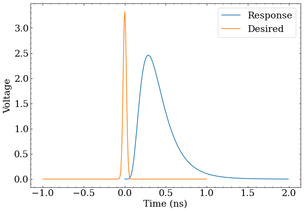
The response function of a photon detector, and the desired pulse shapes after deconvolution.
Now it’s time to produce the the “filter” function $k’(t)$ to convolve with the a signal to deconvolve (transform) “response” into “desired”.
resp_f = np.fft.fft(resp_y)
desire_f = np.fft.fft(desire_y)
filter_f = desire_f/resp_f

time_step = (x[1]-x[0])
filter_y = np.real(np.fft.ifft(filter_f))
filter_x = np.arange(len(filter_y))*time_step
Here, fft computes the Fourier transform, while ifft does the inverse.
The result are filter_x and filter_y representing the samples of $k’(t)$.
Before looking directly at the filter function, have a look at the power spectrum of these three functions.
Power is the square of the amplitude, which for complex numbers is given by $|x|^2$.
Numpy has a convenient fftfreq function to calculate the frequency associate with each index of the FFT result.
Note that Fourier transforms include positive and negative frequencies, but as these are the same for these power spectra, I’ll only show the positive component.
ps_resp = np.abs(resp_f)**2
ps_desire = np.abs(desire_f)**2
ps_filter = np.abs(filter_f)**2

freqs = np.fft.fftfreq(resp_y.size, time_step/1e9)
idx = np.argsort(freqs)
idx = idx[freqs[idx]>=0]

plt.plot(freqs[idx], ps_resp[idx],label='Response')
plt.plot(freqs[idx], ps_desire[idx],label='Desired')
plt.plot(freqs[idx], ps_filter[idx],label='Filter')
plt.yscale('log')
plt.xlabel('Freq (Hz)')
plt.ylabel('Power')
plt.legend()

The power spectra of the response, desired, and deconvolution filter. Deconvolution never looked simpler…
Examining this, it appears that the primary effect of the deconvolution filter will be to boost frequencies in the 8-35 GHz range (roughly) with maximal boosting around 20 GHz, and reduce frequencies outside of this range. Since a reduction of low frequencies and boosting of higher frequency would be required to transform a wide pulse into a more narrow pulse, this makes some conceptual sense.
Recall the discussion about transforming a response into a delta function having undesirable features. The resulting filter power function would be a reflection of the response function about $10^0$ on this log plot, generally increasing instead of trailing off strongly at higher frequencies. This would behave poorly in almost any scenario.
Going back to the practical filter function, the time-domain $k’(t)$ can now be plotted easily.
plt.plot(filter_x,filter_y,label='Deconv. Filter')
plt.ylabel('Unitless')
plt.xlabel('Time (ns)')
plt.legend()
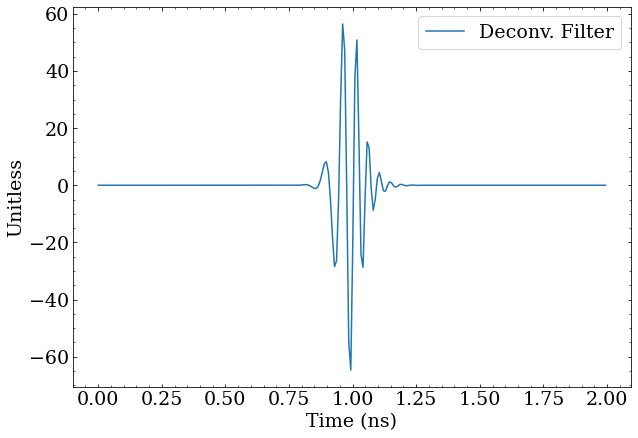
The resulting deconvolution filter, which deconvolves the response into the desired pulse shape when convolved with a signal. Not confusing at all!
This structure appears very mysterious at a glance, but those familiar with quantum mechanics might recognize this shape as being similar to a wave packet, which is only coincidental, and due to both having (approximately) Gaussian distributions in the frequency domain. The width of the filter envelope is roughly related to the width of the response function, while the higher frequency is related to the width of the desired function. A bit more intuition is found here regarding the infinitely thin delta function and its reliance on infinite frequencies.
Frankly, it is not obvious at all that convolving this function with a signal would do anything useful, but the proof is in the demonstration. A function that generates a signal with pulses at certain times, convolves it with the filter function, and shows the true times of the pulses is straightforward.
def demo(times):
    y = pulses_at(x,times)
    plt.plot(x,y,label='Signal')
    deconv_y = np.convolve(y,filter_y,'same')
    plt.plot(x,deconv_y,label='Deconvolved')
    plt.scatter(times,np.zeros_like(times),marker='o',c='r',zorder=10)
    plt.ylabel('Voltage')
    plt.xlabel('Time (ns)')
    plt.legend()
Using Placing pulses so close together that they overlap into one bigger pulse with When pulses exactly overlap, such as at 2 ns with Generating random pulses with ![Using demo([1,3]) to generate a pulse at 1 ns and 3 ns, one can see by the placement of the red dots that the deconvolution put a “desired” pulse exactly where the red dot indicates the true pulse was generated.](/images/deconv_demo_simple.png)
demo([1,3]) to generate a pulse at 1 ns and 3 ns, one can see by the placement of the red dots that the deconvolution put a “desired” pulse exactly where the red dot indicates the true pulse was generated.![Placing pulses so close together that they overlap into one bigger pulse with demo([3,3.1]) still results in two distinct “desired” pulses at the correct times.](/images/deconv_demo_overlap.png)
demo([3,3.1]) still results in two distinct “desired” pulses at the correct times.![When pulses exactly overlap, such as at 2 ns with demo(times=[2,2,3]), the “desired” pulses will also overlap, and the integral will be proportional to the number of overlapping pulses. This means photons can still be counted with the integral of the deconvolved signal, and that the width of the “desired” pulse must be chosen such that it’s narrow enough to distinguish photons that can’t be considered to arrive at the same time.](/images/deconv_demo_pileup.png)
demo(times=[2,2,3]), the “desired” pulses will also overlap, and the integral will be proportional to the number of overlapping pulses. This means photons can still be counted with the integral of the deconvolved signal, and that the width of the “desired” pulse must be chosen such that it’s narrow enough to distinguish photons that can’t be considered to arrive at the same time.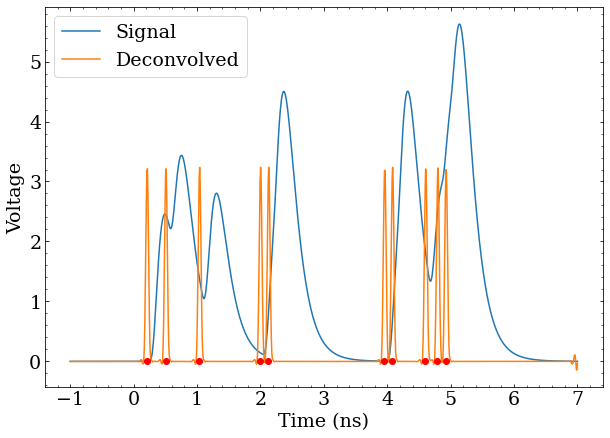
demo(np.random.random(10)*5) further demonstrates that deconvolution is a robust solution to identifying photon arrival times.
The bottom line here is that deconvolution can transform the hard problem of identifying the start times of potentially overlapping pulses into a much easier problem of identifying several discrete features in a signal, perhaps with just a simple threshold. This technique can also be performed without having to do an “online” FFT of data, but rather by convolving data with a filter derived from Fourier analysis of the response function, which is potentially a useful approach for embedding such an analysis into FPGAs or analog pulse processing chips.
>> Home