I was reading an article about scientists who created an accurate simulation of the behavior of simple cells, to really understand their dynamics, and I wondered whether it would be possible to do the same for “simple” atoms or molecules. Some quick exploration into the topic indicates that’s a fairly difficult problem, not to mention an area of active research for multi-electron atoms and simple molecules alike. That said, I can certainly take a stab at some simpler simulations and see how far it can scale up, which should result in some interesting visualizations at the very least.
Not a crash course introduction to quantum mechanics
I’m going to mostly assume you know something about quantum mechanics here, but will try to provide some intuition to the mathematics and focus on concepts. To tie it back to the real science that is quantum mechanics, and develop the simulation, it’s impossible to avoid the math entirely.
Wave functions
Most formulations of quantum mechanics describes particles as complex wave functions, or complex fields, $\psi$, which have some kind of value at every point in space $\vec{x}$. Using a simple one-dimensional space, $\psi(\vec{x})$ is just a regular mathematical function of one real variable, which returns a complex number (see a previous aside on complex numbers). The usual interpretation of quantum mechanics may disagree, but the thinking these days (especially in quantum field theory) is that the wave function is the physically real object here. At the very least, the wave function conclusively describes the chance to detect the particle according to a probability distribution
$$ P(\vec{x}) = \psi^*(\vec{x})\psi(\vec{x}) = \left|\psi(\vec{x})\right|^2 $$
where the ${}^*$ denotes a complex conjugate, or negating the imaginary part of the number, and the whole operation is equivalent to getting the magnitude squared of the complex numbers. This probabilistic interpretation requires that the following be true:
$$ \int \left|\psi(\vec{x})\right|^2\,\,d\vec{x} = 1 $$
meaning the total magnitude of the complex field is 1, conserving probability.
Time evolution
The purpose of quantum mechanics is to describe how wave functions change as a function of time, $\psi(\vec{x},t)$. This is captured by the Schrodinger equation, which I’ll present here in its most general form with no derivation. $$ i\hbar \frac{d\psi(\vec{x},t)}{dt} = \hat{H}\psi(\vec{x},t) $$ Here, $\hat{H}$ is called the Hamiltonian operator and essentially measures, or specifies, the energy of a wave function. Namely, the energy of a wave function is the expectation value of the Hamiltonian, which physicists write as $$ E = \left<\hat{H}\right> = \int \psi^*(\vec{x})\hat{H}\psi(\vec{x})\,\,d\vec{x} $$ which can be thought of as a weighted average of the Hamiltonian applied to the wave function everywhere.
Thinking of the Schrodinger equation as something one might simulate, one might rearrange it to isolate the time derivative $$ \frac{d}{dt} \psi(\vec{x},t) = -\frac{i}{\hbar}\hat{H}\psi(\vec{x},t) $$ which, if we assume the operator $\hat{H}$ is a simple number analogous to energy, says the rate of change of the wave function is proportional to $-i$ times the wave function, itself. This $-i$ factor can be a bit curious, if you’re not very familiar with complex numbers, but multiplying a complex number by something purely imaginary rotates the phase by 90 degrees, and a complex number whose derivative is 90 degrees out of phase simply rotates (changes phase) as a function of time. If the operator $\hat{H}$ includes any imaginary component, that additional phase will be added into the derivative, making it somewhat different than 90 degrees out of phase, which results in a wave function that changes magnitude (as well as phase) over time. This means there are two classes of solution, in general:
- Solutions where the magnitude of the wave function is fixed in time, and only the phases change.
- Solutions where the magnitude and phase of the wave function changes in time.
Operators, and convenient notation
It’s important to recognize that the hat on the Hamiltonian denotes an “operator”. Operators are like functions of wave functions, which return another wave function. These are not often written like functions taking an argument, $\hat{H}(\psi(\vec{x},t))$, but as a function accepting an argument from the right in what appears to be a multiplication, $\hat{H}\psi$, where I’ve employed another notational convenience, and stopped putting function arguments on wave functions. While I’m at it, I choose units where all pesky constants like $\hbar$ are exactly $1$, and stop writing them. Using this convention, one would often write the above equations this way:
$$ i \frac{d\psi}{dt} = \hat{H}\psi $$ $$ E = \left<\hat{H}\right> = \int \psi^*\hat{H}\psi\,\,d\vec{x} $$
But remember: this isn’t just regular scalar multiplication! Like multiplication by matrices, application of operators to wave functions does not commute, which means in general $$ \hat{H}\psi \neq \psi\hat{H} $$ though, there are special cases where this may be true.
General solutions to time evolution
The Schrodinger equation says that the rate of change of the wave function is related to the energy of said wave function. Indeed, there are certain special wave functions $\phi(\vec{x})$, called eigenstates, which satisfy the following relationship $$ \hat{H}\phi = E\phi $$ meaning the result of the Hamiltonian operating on $\phi$ is the same wave function $\phi$ scaled by a fixed energy $E$. This places significant constraints on what $\phi$ can be, which depends on exactly what the Hamiltonian is. From the Schrodinger equation, it’s clear that eigenstates of the Hamiltonian will satisfy $$ \frac{d\phi}{dt} = -i E \phi $$
The solution to this is any function proportional $e^{-iEt}$, which shows that $$ \phi(\vec{x},t) = e^{-iEt}\phi(\vec{x}) $$ meaning only the complex phase of the eigenstates change with time, which is the class 1 solutions mentioned above.
It is also a consequence of group theory that the set of all such eigenstates $\phi_n$ form a complete basis, meaning any wave function $\psi$ can be written as a combination, or superposition, of such eigenstates with time-dependent complex coefficients. $$ \psi(\vec{x},t) = \sum_n C_n(t) e^{-iE_nt} \phi_n(\vec{x}) $$ The coefficients may simply be constants, or be functions of time (for systems with more complicated dynamics). These superpositions are the general class 2 solutions above.
Typical treatments of quantum mechanics abandon the general wave functions here, and opt for the more mathematically-tractable eigenstates, handwaving that all real wave functions are just linear superpositions of the special eigenstates. The eigenstates will come up a bit later, but I’ll instead opt for a more holistic treatment of general wave functions.
Specifics: a single particle Hamiltonian
The simplest case that is taught to students first learning quantum mechanics is of a particle in one dimension. This isn’t a severe approximation, as it is relatively straightforward to generalize this to higher dimensions, and most important points can be demonstrated in this simpler case. The Hamiltonian is supposed to calculate energy from a wave function and in the case of a single particle there’s only two energies to consider: the kinetic energy of the particle, and any potential energy it may experience.
$$ \hat{H} = \hat{K} + \hat{V} $$
Here, $\left<\hat{K}\right>$ is the kinetic energy of the wave function, and $\left<\hat{V}\right>$ is the potential energy. The potential energy can be any function of space, and simply scales the wave function it operates on by some position-dependent value $V(\vec{x})$ or just $V$ to save characters.
The kinetic energy must extract the momentum of the wave in the wave function to compute the classical $\frac{p^2}{2m}$ where $p$ is the momentum and $m$ is the mass of the particle. Letting $\hat{p}$ become a momentum operator, we can now write
$$ \hat{H} = \frac{1}{2m}\hat{p}^2 + V $$
where a squared operator means to apply it twice in a row to whatever is to the right.
Now for the question of how to extract momentum from a wave function. The probability of detecting a particle is the magnitude of the complex wave function, but the momentum is encoded in the rate of change of phase of the complex numbers with respect to position, or the imaginary part of $\frac{d\psi}{dx}$. This can be made clear if $\phi$ is further restricted to being an eigenstate of the momentum operator $$ \hat{p}\phi = p\phi $$ We can then say three things about the form of momentum operator, if we consider a Hamiltonian with no potential:
- The result of applying the momentum operator to a momentum eigenstate must be proportional (by $p$) to the eigenstate.
- The momentum eigenstate is an eigenstate of the Hamiltonian as well, and therefore only the phase, not the magnitude, changes in time. That phase change is proprtional to $p^2$.
- A state with momentum but constant magnitude must have the same magnitude everywhere in space, by symmetry, meaning spatial derivatives should have no real component.
This implies that the momentum operator is takes an imaginary spatial derivative to a real number $$ \hat{p} = -i\frac{d}{dx} $$ where the $-i$ factor converts the derivative of the purely-rotating complex number, which is 90 degrees out of phase, back into a complex number proportional to the original value. Therefore, $$ \hat{p}^2 = -\frac{d^2}{dx^2} $$ where we should recall that I’m dropping most constants like $\hbar$.
The final result is the Hamiltonian $$ \hat{H} = \frac{-1}{2m}\frac{d^2}{dx^2} + V $$ and the Schrodinger equation $$ \frac{d\psi}{dt} = -i \left(\frac{-1}{2m}\frac{d^2}{dx^2} + V\right) \psi $$
$$ \frac{d\psi}{dt} = \frac{i}{2m}\frac{d^2}{dx^2}\psi - iV\psi $$ which, considering the factor of $i$ means the momentum squared (energy, or second derivative of the phase as a function of position) serves to rotate the phase in time, while the second derivative of the magnitude as a function of position (for more general wavefunctions than momentum eigenstates) serves to change the magnitude of the wave function in time.
In the end, this complicated interplay lets the Schrodinger equation move probability around according to the momentum encoded in the wave function, and critically lets the Schrodinger equation generate momentum in the wave function whenever there are spatial gradients in probability. To believe this, one really has to see it in action.
Towards a numerical simulation
To start with simulating and visualizing some quantum mechanics, one needs to represent a wave function, use the Schrodinger equation to find its time derivative, step the wave function forward in time, and repeat. As wave functions are entities with a complex value at every point in space mathematically this is usually represented as a continuious function $\psi(\vec{x})$ mapping points in space to complex values. There’s an infinite amount of information contained in said function, but we don’t need it all, and can instead represent an approximate wave function by tracking complex numbers $\psi_j$ at discrete points on some spatial grid given by points $\vec{x}_j$.
Nominally, one could think of the true $\psi(\vec{x})$ as being interpolated from the grid of $\psi_j$, meaning any features in $\psi(\vec{x})$ smaller than the grid size will be lost. This effectively puts an upper limit on the momentum the wave function can encode, since momentum is a change in phase w.r.t. position, and lower limit on precision of position that can be represented. Those familiar with the uncertainty principle will see it here, where very precise positions imply very high momentum. Critically, one can make the grid spacing sufficiently small to approximate the dynamics of any system, at the cost of having to store more information about the system.
The Schrodinger equation can be rewritten to use this approximation of the wave function
$$ \frac{d}{dt}\psi_j = \frac{i}{2m}\frac{d^2}{dx^2}\psi_j - iV\psi_j $$
where now it looks as if there are now $j$ Schrodinger equations, one for each point! This is actually a perfectly reasonable interpretation, which would be even more palatable had I done a more rigorous discretization of space, hypothesizing that $\vec{x}_j$ represents certain allowed positions for particles to be in. The final remaining weirdness is an apparent second derivative of spatial coordinates of the $\psi_j$. In discretizing the wave function, one must also discritize the spatial derivative into a finite difference.
$$ \frac{d^2}{dx^2} \psi(\vec{x}) \rightarrow \frac{1}{\Delta x}(\psi_{j-1} - 2 \psi_{j} + \psi_{j+1}) $$ Here, $\Delta x$ is the grid spacing, which I’ll drop like most other scale factors.
Now the Schrodinger equation can truly be written as $j$ coupled differential equations $$ \frac{d}{dt}\psi_j = \frac{i}{4m}( \psi_{j-1} - 2 \psi_{j} + \psi_{j+1} ) - iV\psi_j $$ where it is plainly evident that difference in magnitude and phase adjacent to a point impact the dynamics at that point, and it takes time for any local disturbance to propagate to further points.
We’ve arrived at an expression that can be simulated fairly easily. $\psi_j$ represents the wave function sampled on a grid of uniformly spaced points, and a discrete Schrodinger equation specifies how sampled wave function value should change as a function of adjacent points. Let’s get to the code.
Discrete wave functions
All the discrete wave functions used where will be sampled at the same set of spatial points x.
import numpy as np
x = np.linspace(-10,10,5000)
deltax = x[1]-x[0]
Any complex vector phi of the same shape as x is a valid wave function, but to keep the probabilistic interpretation of the square of the wave function, we’ll require they be normalized.
def norm(phi):
    norm = np.sum(np.square(np.abs(phi)))*deltax
    return phi/np.sqrt(norm)
It is also highly desirable, for the purposes of blogging, to generate some visualizations of said wave functions.
def complex_plot(x,y,prob=True,**kwargs):
    real = np.real(y)
    imag = np.imag(y)
    a,*_ = plt.plot(x,real,label='Re',**kwargs)
    b,*_ = plt.plot(x,imag,label='Im',**kwargs)
    plt.xlim(-2,2)
    if prob:
        p,*_ = plt.plot(x,np.abs(y),label='$\sqrt{P}$')
        return a,b,p
    else:
        return a,b
Even in 1D, visualizing complex numbers is a bit of a trick, but I’ve opted to simply plot the real and imaginary components separately, even though the phase and magnitude are the more intuitive quantities. To help with this, it’s optional to plot the magnitude as well, which is the square root of the probability to find a particle.
Finally, to simulate something, we need a starting point. A wave function that is zero everywhere makes the statement that there is no particle at all, so that won’t do. Instead, let’s take an educated stab in the dark and assume the particle has some normal probability distribution, and optionally has some momentum, which I’ll suggestively call a wave packet.
def wave_packet(pos=0,mom=0,sigma=0.2):
    return norm(np.exp(-1j*mom*x)*np.exp(-np.square(x-pos)/sigma/sigma,dtype=complex)
The normal distribution part is a typical $e^{-(x-\mu)^2/\sigma^2}$, while the momentum is encoded as change in phase w.r.t. position with $e^{-ipx} = \sin(px)+i \cos(px)$.
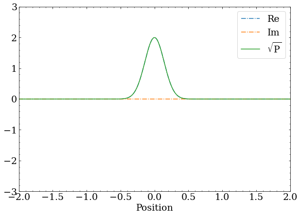
A wave packet with zero momentum is just a real-valued Gaussian distribution. The square root of the probability is identical to the real component of the complex wave function.
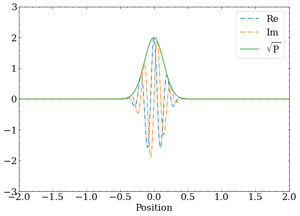
A wave packet with nonzero momentum still has a magnitude that is a Gaussian distribution, but the complex phase changes as a function of position at a rate proportional to the momentum.
Implementing discrete time evolution
To compute Schrodinger’s equation and time evolve a wave function, first a method to compute second spatial derivative is needed.
def d_dxdx(phi,x=x):
    dphi_dxdx = -2*phi
    dphi_dxdx[:-1] += phi[1:]
    dphi_dxdx[1:] += phi[:-1]
    return dphi_dxdx/deltax
I’ve imposed some boundary conditions on the ends here, which basically fixes points on the wave function to the right and left of the sampling space to zero.
The rest of the Schrodinger equation, for computing the time derivative of the wave function, follows, with some constants restored.
def d_dt(phi,h=1,m=100,V=0):
    return 1j*h/2/m * d_dxdx(phi) - 1j*V*phi/h
Now, for the actual time evolution, we can consider the simplest case of Euler’s method $$ \psi(t+\Delta t) = \psi(t) + \Delta t \frac{d\psi(t)}{dt} $$ which is reasonably correct for small enough $\Delta t$, and is easy to implement.
def euler(phi, dt, **kwargs):
    return phi + dt * d_dt(phi, **kwargs)
However, I don’t want to wait forever taking tiny $\Delta t$ steps. Better integration techniques essentially estimate the average derivative over the timestep better than assuming it’s the derivative at the current time, and therefore have less error overall, allowing for larger time steps. A 4th order Runge-Kutta integrator is my goto.
def rk4(phi, dt, **kwargs):
    k1 = d_dt(phi, **kwargs)
    k2 = d_dt(phi+dt/2*k1, **kwargs)
    k3 = d_dt(phi+dt/2*k2, **kwargs)
    k4 = d_dt(phi+dt*k3, **kwargs)
    return phi + dt/6*(k1+2*k2+2*k3+k4)
A full simulation
Now for a generic method to step a wave function through time, saving results periodically for visualization purposes.
def simulate(phi_sim,
             method='rk4',
             V=0,
             steps=100000,
             dt=1e-1,
             condition=None,
             normalize=True,
             save_every=100):
    simulation_steps = [np.copy(phi_sim)]
    for i in range(steps):
        if method == 'euler':
            phi_sim = euler(phi_sim,dt,V=V)
        elif method == 'rk4':
            phi_sim = rk4(phi_sim,dt,V=V)
        else:
            raise Exception(f'Unknown method {method}')
        if condition:
            phi_sim = condition(phi_sim)
        if normalize:
            phi_sim = norm(phi_sim)
        if save_every is not None and (i+1) % save_every == 0:
            simulation_steps.append(np.copy(phi_sim))
    return simulation_steps
This has several optional arguments to change the dynamics.
A potential energy, which I’ll get to later, can be specified with V.
The length of the simulation can be controlled with dt and steps, with the wave function stored each save_every steps to be returned.
Finally, there’s an option to disable normalizing the state after each step, and a placeholder to apply some condition that mutates the wave function at each step.
On the point of normalization - nominally a quantum Hamiltonian will preserve total probability, and an exact mathematical treatment has this property. This numerical approach, however, only approximately conserves probability, which could lead to numerical instability if left unchecked. A much more stable simulation is achieved if we require that the wave function at each time step be normalized.
Visualizing the dynamics
With all the formalism and simulation framework out of the way, only the cool visualizations remain.
Looking at the wave_packet developed earlier, simulate can produce a series of time steps showing the evolution of the wave function,
sim_free = simulate(wave_packet(),steps=200000,plot_every=None,save_every=1000)
Some futzing around with matplotlib’s animation API suggests I can create animations of this time evolution with something like the following.
from matplotlib.animation import FuncAnimation

def animate(simulation_steps,init_func=None):
    fig = plt.figure()
    re,im,prob = complex_plot(x,simulation_steps[0])
    plt.xlim(-2,2)
    plt.ylim(-2,2)
    if init_func:
        init_func()
    plt.legend()

    def animate(frame):
        prob.set_data((x, np.abs(simulation_steps[frame])))
        re.set_data((x, np.real(simulation_steps[frame])))
        im.set_data((x, np.imag(simulation_steps[frame])))
        return prob,re,im

    anim = FuncAnimation(fig, animate, frames=int(len(simulation_steps)), interval=50)
    plt.close()

    return anim
And a simple call to animate(sim_free) gives a nice visualization of how the wave function changes with time.
This demonstrates a foundational result of quantum mechanics, which is that the width of a Gaussian wave packet grows with time. How does this happen? The second derivative of the magnitude of the wave function induces the phase to change, and since the second derivative is not constant (derivative of a Gaussian is a Gaussian), the rate of phase change is not constant, leading to a winding phase. The winding phase represents momentum away from the particle origin, which induces the probability to spread out over time.
Why does this happen? The zero momentum wave packet, or any wave function, is really composed of a superposition of momentum eigenstates. At the instant in time that there is a stationary probability distribution, it’s a careful balance of positive and negative momentum states. As the state evolves, the momentum states start to depart the origin in opposite directions in order of highest momentum, causing the wave function to spread out
A wave packet with some momentum can be simulated as well, starting from wave_packet(mom=10).
Here, the spreading of the wave function still occurs, but the bulk distribution is also moving in the direction of positive momentum, since the state is now largely composed of momentum eigenstates with positive momentum.
Considering interactions
That’s about all there is to look at for one dimensional free particles, but we can now consider a particle that interacts with some external potential, which will modify the dynamics. The potential $V$ here refers to the energy necessary for a particle to simply be in a location. In the time derivative from the Schrodinger equation, the potential energy enters in with the opposite 90 degree phase rotation as the momentum squared, which means a potential in a region tends to reduce the momentum in a wave function that tries to enter into that region, and a very large potential can completely prevent a wave function from having nonzero probability in a region. Importantly, a large enough opposing value of the potential in the derivative will reverse the momentum, and send the particle in the opposite direction, picking up momentum instead of slowing down. This is exactly the classical interpretation of how potential energy affects particles, and a few simple cases can be explored.
A particle in a box
The simplest of potentials to consider is zero within a region and infinite (or sufficiently large) outside that region. This is the typical “particle in a box” problem, which is often explored because its eigenstates are easy to tease out analytically. Putting eigenstates aside for now, the same wave packet with momentum can be simulated within such a potential, as long as it is specified. I’ll let the potential between (-2,2) be zero, and one (which in these units is huge) elsewhere.
box_potential = np.where((x>-2)&(x<2),0,1)
sim_box_mom = simulate(wave_packet(mom=10),V=box_potential,steps=100000,save_every=500)
I’ll also make use of the init_func in animate to add some red shading to the disallowed region.
def box_init():
    plt.gcf().axes[0].axvspan(2, 3, alpha=0.2, color='red')
    plt.gcf().axes[0].axvspan(-3, -2, alpha=0.2, color='red')
    plt.xlim(-3,3)
    plt.ylim(-3,3)
This has the qualitative behavior you might expect from a particle with some momentum in a box: it hits a wall and bounces back. The wave packets still spreads out over time, and near the bounces we start to see interference patterns as the reflected part of the packet interferes with the part that hasn’t reflected yet. These bumpy interference fringes in the probability are a purely quantum mechanical effect, and has no classical analogue for massive particles, which is a measurable way to verify quantum mechanics is an accurate description of reality.
A particle encounters a barrier
The particle in a box example shows how particles react to impassable barriers, but what if the barrier is only difficult to pass? A real life example here is the effect known as quantum tunneling, which is critical for life-giving processes like nuclear fusion in the Sun. Protons, on average, do not have enough energy, even in the Sun, to overcome the repulsion of other protons entirely. However, some component of the quantum mechanical protons do make it past the potential barrier presented by the other protons, and thus there is light. An analogue of this tunneling process can be demonstrated in one dimension, by shooting a wave packet at a finite region of potential that is slightly higher than the energy of the particle.
Tweaking the barrier strength to get a reasonable visualization, I arrived at:
barrier_weak_potential = np.where((x>1.4)&(x<1.6),3.5e-2,0)
sim_barrier_mom = simulate(wave_packet(mom=10),V=barrier_weak_potential,steps=50000,save_every=500)

def barrier_init():
    plt.gcf().axes[0].axvspan(1.4, 1.6, alpha=0.2, color='orange')
    plt.xlim(-2,4)
    plt.ylim(-3,3)
animate(sim_barrier_mom,init_func=barrier_init)
Notice that, within the region of the potential, the wave function is not oscillatory, but rather exponentially damped, which is what a rigorous treatment of this situation would show. This is because there is not enough kinetic energy for a classical particle to enter this potential, at all, but the boundary conditions of the quantum mechanical wave function are such that it does penetrate some depth into classically forbidden regions. As the potential increases, this penetration depth decreases.
The quantum tunneling effect occurs when the width of the barrier is comparable, or less than, the penetration depth. If any of the probability makes it through to a low enough potential region, it continues on as a regular wave packet. The physical interpretation here is that even though the particle’s energy is insufficient, the higher momentum eigenstates that help localize it do have enough energy to pass the barrier. Indeed, the wave packet that passes (reflects) has higher (lower) momentum than the initial packet!
A particle in a quadratic potential
Considering a “quantum spring” with a restoring force proportional to the distance from the origin, $\vec{F} = -A\vec{x}$, it is well know the potential is quadratic $V = \frac{1}{2}Ax^2$. The reality is that any potential is approximately quadratic near enough to its minimum, so understanding the quadratic potential $Ax^2$, often called a quantum harmonic oscillator, has wide applications in real problems.
Again, tweaking the potential strength for a nice visualization:
quadratic_potential = 1e-2*np.square(x)
sim_quadratic_potential = simulate(wave_packet(mom=10),V=quadratic_potential,steps=400000,save_every=500)

def quadratic_init():
    plt.fill_between(x,(np.square(x)-3),-3,color='orange',alpha=0.2)
    plt.xlim(-3,3)
    plt.ylim(-3,3)
animate(sim_quadratic_potential,init_func=quadratic_init)
Notice that this, unlike the particle in a box, is periodic. Anyone who has worked with quadratic potentials or masses on spring should know this: the amplitudes of states with different momentum are different, but the period of the oscillation is the same for all. So, higher lower momentum components of the wave function go further from the origin, giving wider probability distributions at the edge of the oscillation, but they all sync back up near the origin.
It is also plainly clear here that densely wound phases correspond to faster moving states, since the density is greatest near the middle, and the wave packet is briefly (instantaneously) all the same phase when it’s stationary at the edges.
An aside on Eigenstates
This simulation framework is fun to generate visualizations with, but it can also be used to do real science by finding the ground and excited states of systems. This can be done by exploiting a technique called imaginary time evolution. Essentially, simply replacing $\Delta t$ with $-i \Delta t$ in the simulation and propagating into “imaginary time” will damp out all but the lowest energy eigenstates. How this works is pretty self evident if we look back at the expression for a general wave function in terms of eigenstates. $$ \psi(\vec{x},t) = \sum_n C_n(t) e^{-iE_nt} \phi_n(\vec{x}) $$ Letting $t \rightarrow -it$ transforms this equation into $$ \psi(\vec{x},t) = \sum_n C_n(t) e^{-E_nt} \phi_n(\vec{x}) $$ where each eigenstate is now exponentially damped by $e^{-E_n t}$, which goes to zero at infinite $t$. Critically, this factor goes to zero faster for higher energy states, meaning the lowest energy state is the last to disappear.
So, if we require that the wave function remain normalized, which the simulate method already does, simply evolving in imaginary time will damp out all but the lowest energy eigenstate.
The eigenstates of the particle in a box are easy enough for the initiated to remember (simply all sinusoidal functions that go to zero at the edges), but the expression for the eigenstates of the quantum harmonic oscillator are complicated enough to have to look up the analytical form and still feel a little confused each time, so let’s just generate those from the simulation.
As I’ve alluded to several times, the wave packet I’ve been using is a broad superposition of many eigenstates, so chances are the ground state is in there to some degree.
sim_quad_0 = simulate(wave_packet(mom=10),dt=-1e-1j,V=quadratic_potential,steps=200000,save_every=1000)
animate(sim_quad_0,init_func=quadratic_init)
Note that the imaginary time evolution quickly damps out the momentum, and the result is some stationary Gaussian that is a bit wider than the initial wave packet. Fortunately for my narrative, the ground state of the QHO is exactly a Gaussian with a width determined by the strength of the potential.
To generate an excited state, in principle, one could take any wave packet $\psi$, remove the ground state $\phi_0$ from it (i.e. set it’s $C_0(t)$ coefficient to zero), and perform the same procedure on the resulting $\Psi_1$ to find the first excited eigenstate $\phi_1$. $$ \Psi_1 = \psi - \left( \int \phi_0^* \psi \,\, dx \right) \phi_0 = \psi - C_0(t)\phi_0 $$ Here the integral is used to determine the complex coefficient weight of $\phi_0$ within $\psi$. This works because the eigenstates have an orthogonality property of zero overlap $$ \delta_{nm} = \int \phi_n^* \phi_m \,\, dx $$ where $\delta_{nm}$ is one if $n=m$ and zero otherwise.
psi = wave_packet(mom=10)
phi_0 = sim_quad_0[-1]
Psi_1 = psi - np.sum(np.conjugate(phi_0)*psi)*deltax*phi_0
complex_plot(x,Psi_1)
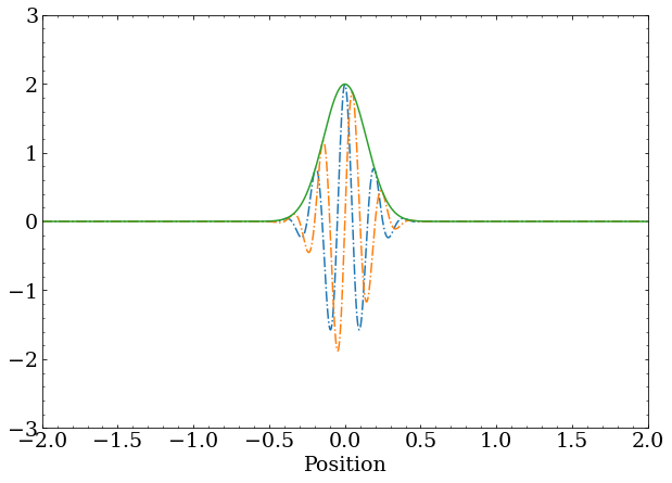
The same wave packet with momentum shown throughout this post, but this time with the ground state of the quantum harmonic oscillator removed. You’re right - it doesn’t look very different. The coefficient of the ground state in the initial superposition was small, but nonzero, so removing it doesn’t significantly change the wave function.
The problem, of course, is numerical stability. The found ground state is arbitrarily close to the real ground state, but not close enough to completely remove all of the lowest energy eigenstate from the wave packet.
What’s worse, numerical instability in integrating the Schrodinger equation will invariably put some infinitesimal probability back into the ground state, causing it imaginary time evolution to once again collapse to it.
The canonical (quick and dirty) solution to this problem is to simply remove the ground state from the wave function after each time step, to ensure its coefficient stays approximately zero, and then normalizing the wave function again.
This is why I added the condition option to the simulate function — I’ll pass a function here to remove $\phi_0$ at each time step.
def orthogonal_to(states):
    def orthogonalize(phi):
        for state in states:
            phi = phi - np.sum(np.conjugate(state)*phi)*deltax*state
        return phi
    return orthogonalize

sim_quad_1 = simulate(Phi_1, dt=-1e-1j, condition=orthogonal_to([phi_0]), V=quadratic_potential, steps=200000, save_every=1000)
animate(sim_quad_1,init_func=quadratic_init)
The complex squiggle and double peaked probability is exactly what the first excited eigenstate looks like. The same procedure, removing the ground and first excited state and evolving with imaginary time, can build up the next excited state ad infinitum.
Now, you might ask yourself how to verify that these states are in fact eigenstates without having to look up and plot the analytic solutions to the QHO, and the answer is simple: evolve it in time, and only the phase should change!
Until next time…
And that’s it for this post! I have generalized this framework to three dimensions and included GPU acceleration with Cupy to deal with the significantly larger number of calculations required, but the qualitative results are the same. If I have time, perhaps I will look at Hydrogen like atoms, to extract orbitals (eigenstates!), or even slightly more complicated atomic systems. This gets difficult fast because each electron experiences the Coulomb force from both the nucleus and the other electrons, and there’s the spin of the electrons and Pauli exclusion principle to deal with. Needless to say, this exercise has convinced me that the aspiration to simulate simple atomic or molecular system in some general way with quantum mechanics is, in fact, quite difficult!
>> Home